Chapter 25. Profiling and optimization
Table of Contents
Haskell is a high level language. A really high level language. We can spend our days programming entirely in abstractions, in monoids, functors and hylomorphisms, far removed from any particular hardware model of computation. The language specification goes to great lengths to avoid prescribing any particular evaluation model. These layers of abstraction let us treat Haskell as a notation for computation itself, letting the programmer concentrate on the essence of their problem without getting bogged down in low level implementation decisions. We get to program in pure thought.
However, this is a book about real world programming, and in the real world, code runs on stock hardware with limited resources. Our programs will have time and space requirements that we may need to enforce. As such, we need a good knowledge of how our program data is represented, the precise consequences of using lazy or strict evaluation strategies, and techniques for analyzing and controlling space and time behavior.
In this chapter we'll look at typical space and time problems a Haskell programmer might encounter, and how to methodically analyse, understand and address them. To do this we'll use investigate a range of techniques: time and space profiling, runtime statistics, and reasoning about strict and lazy evaluation. We'll also look at the impact of compiler optimizations on performance, and the use of advanced optimization techniques that become feasible in a purely functional language. So let's begin with a challenge: squashing unexpected memory usage in some inoccuous looking code.
Profiling Haskell programs
Let's consider the following list manipulating program, which naively computes the mean of some large list of values. While only a program fragment (and we'll stress that the particular algorithm we're implementing is irrelevant here), it is representative of real code we might find in any Haskell program: typically concise list manipulation code, and heavy use of standard library functions. It also illustrates several common performance trouble spots that can catch out the unwary.
-- file: ch25/A.hs
import System.Environment
import Text.Printf

main = do
    [d] <- map read `fmap` getArgs
    printf "%f\n" (mean [1..d])

mean :: [Double] -> Double
mean xs = sum xs / fromIntegral (length xs)
This program is very simple: we import functions for accessing the
system's environment (in particular, getArgs), and the
Haskell version of printf, for formatted text output.
The program then reads a numeric literal from the command line, using that to
build a list of floating point values, whose mean value we compute by
dividing the list sum by its length. The result is printed as a string. Let's
compile this source to native code (with optimizations on) and run it with
the time command to see how it performs:
$ghc --make -O2 A.hs[1 of 1] Compiling Main ( A.hs, A.o ) Linking A ...$time ./A 1e550000.5 ./A 1e5 0.05s user 0.01s system 102% cpu 0.059 total$time ./A 1e6500000.5 ./A 1e6 0.26s user 0.04s system 99% cpu 0.298 total$time ./A 1e75000000.5 ./A 1e7 63.80s user 0.62s system 99% cpu 1:04.53 total
It worked well for small numbers, but the program really started to struggle with input size of ten million. From this alone we know something's not quite right, but it's unclear what resources are being used. Let's investigate.
Collecting runtime statistics
To get access to that kind of information, GHC lets us pass flags directly to
the Haskell runtime, using the special +RTS and
-RTS flags to delimit arguments reserved for the runtime system.
The application itself won't see those flags, as they're immediately consumed
by the Haskell runtime system.
In particular, we can ask the runtime system to gather memory and garbage
collector performance numbers with the -s flag (as well as
control the number of OS threads with -N, or tweak the
stack and heap sizes). We'll also use runtime flags to enable different
varieties of profiling. The complete set of flags the Haskell
runtime accepts is documented in the
GHC User's Guide:
So let's run the program with statistic reporting enabled, via +RTS -sstderr,
yielding this result.
$./A 1e7 +RTS -sstderr./A 1e7 +RTS -sstderr 5000000.5 1,689,133,824 bytes allocated in the heap 697,882,192 bytes copied during GC (scavenged) 465,051,008 bytes copied during GC (not scavenged) 382,705,664 bytes maximum residency (10 sample(s)) 3222 collections in generation 0 ( 0.91s) 10 collections in generation 1 ( 18.69s) 742 Mb total memory in use INIT time 0.00s ( 0.00s elapsed) MUT time 0.63s ( 0.71s elapsed) GC time 19.60s ( 20.73s elapsed) EXIT time 0.00s ( 0.00s elapsed) Total time 20.23s ( 21.44s elapsed) %GC time 96.9% (96.7% elapsed) Alloc rate 2,681,318,018 bytes per MUT second Productivity 3.1% of total user, 2.9% of total elapsed
When using -sstderr, our program's performance numbers are
printed to the standard error stream, giving us a lot of information about
what our program was doing. In particular, it tells us how much time was
spent in garbage collection, and what the maximum live memory usage was. It
turns out that to compute the mean of a list of 10 million elements our
program used a maximum of 742 megabytes on the heap, and spent 96.9% of its time
doing garbage collection! In total, only 3.1% of the program's running time was
spent doing productive work.
So why is our program behaving so badly, and what can we do to improve it? After all, Haskell is a lazy language: shouldn't it be able to process the list in constant space?
Time profiling
GHC, thankfully, comes with several tools to analyze a program's time and space usage. In particular, we can compile a program with profiling enabled, which, when run, yields useful information about what resources each function was using. Profiling proceeds in three steps: compiling the program for profiling; running it with particular profiling modes enabled; and inspecting the resulting statistics.
To compile our program for basic time and allocation profiling, we use the
-prof flag. We also need to tell the profiling code which
functions we're interested in profiling, by adding "cost centres" to them. A
cost centre is a location in the program we'd like to collect statistics about,
and GHC will generate code to compute the cost of evaluating the expression
at each location. Cost centres can be added manually to instrument any
expression, using the SCC pragma:
-- file: ch25/SCC.hs
mean :: [Double] -> Double
mean xs = {-# SCC "mean" #-} sum xs / fromIntegral (length xs)
Alternatively, we can have the compiler insert the cost centres on all top
level functions for us by compiling with the -auto-all flag.
Manual cost centres are a useful addition to automated cost centre profiling,
as once a hot spot has been identified, we can precisely pin down the
expensive sub-expressions of a function.
One complication to be aware of: in a lazy, pure language like Haskell, values
with no arguments need only be computed once (for example, the large list in
our example program), and the result shared for later uses. Such values are not
really part of the call graph of a program, as they're not evaluated on each
call, but we would of course still like to know how expensive their one-off
cost of evaluation was. To get accurate numbers for these values, known as
"constant applicative forms", or CAFs, we use the -caf-all flag.
Compiling our example program for profiling then (using the
-fforce-recomp flag to to force full recompilation):
$ghc -O2 --make A.hs -prof -auto-all -caf-all -fforce-recomp[1 of 1] Compiling Main ( A.hs, A.o ) Linking A ...
We can now run this annotated program with time profiling enabled (and we'll use a smaller input size for the time being, as the program now has additional profiling overhead):
$time ./A 1e6 +RTS -pStack space overflow: current size 8388608 bytes. Use `+RTS -Ksize' to increase it. ./A 1e6 +RTS -p 1.11s user 0.15s system 95% cpu 1.319 total
The program ran out of stack space! This is the main complication to be aware
of when using profiling: adding cost centres to a program modifies how it is
optimized, possibly changing its runtime behavior, as each expression now
has additional code associated with it to track the evaluation steps. In a
sense, observing the program executing modifies how it executes. In this
case, it is simple to proceed -- we use the GHC runtime flag, -K,
to set a larger stack limit for our program (with the usual suffixes
to indicate magnitude):
$time ./A 1e6 +RTS -p -K100M500000.5 ./A 1e6 +RTS -p -K100M 4.27s user 0.20s system 99% cpu 4.489 total
The runtime will dump its profiling information into a file,
A.prof (named after the binary that was executed) which
contains the following information:
Time and Allocation Profiling Report  (Final)

	   A +RTS -p -K100M -RTS 1e6

	total time  =        0.28 secs   (14 ticks @ 20 ms)
	total alloc = 224,041,656 bytes  (excludes profiling overheads)

COST CENTRE  MODULE               %time %alloc

CAF:sum      Main                  78.6   25.0
CAF          GHC.Float             21.4   75.0

                                            individual    inherited
COST CENTRE MODULE         no.    entries  %time %alloc   %time %alloc

MAIN        MAIN            1           0   0.0    0.0   100.0  100.0
 main       Main          166           2   0.0    0.0     0.0    0.0
  mean      Main          168           1   0.0    0.0     0.0    0.0
 CAF:sum    Main          160           1  78.6   25.0    78.6   25.0
 CAF:lvl    Main          158           1   0.0    0.0     0.0    0.0
  main      Main          167           0   0.0    0.0     0.0    0.0
 CAF        Numeric       136           1   0.0    0.0     0.0    0.0
 CAF        Text.Read.Lex 135           9   0.0    0.0     0.0    0.0
 CAF        GHC.Read      130           1   0.0    0.0     0.0    0.0
 CAF        GHC.Float     129           1  21.4   75.0    21.4   75.0
 CAF        GHC.Handle    110           4   0.0    0.0     0.0    0.0
This gives us a view into the program's runtime behavior. We can see the program's name and the flags we ran it with. The "total time" is time actually spent executing code from the runtime system's point of view, and the total allocation is the number of bytes allocated during the entire program run (not the maximum live memory, which was around 700MB).
The second section of the profiling report is the proportion of time and space
each function was responsible for. The third section is the cost centre report,
structured as a call graph (for example, we can see that
mean was called from main. The
"individual" and "inherited" columns give us the resources a cost centre was
responsible for on its own, and what it and its children were responsible for.
Additionally, we see the one-off costs of evaluating constants (such as the
floating point values in the large list, and the list itself) assigned to top
level CAFs.
What conclusions can we draw from this information? We can see that the majority of time is spent in two CAFs, one related to computing the sum, and another for floating point numbers. These alone account for nearly all allocations that occurred during the program run. Combined with our earlier observation about garbage collector stress, it begins to look like the list node allocations, containing floating point values, are causing a problem.
For simple performance hot spot identification, particularly in large programs where we might have little idea where time is being spent, the initial time profile can highlight a particular problematic module and top level function, which is often enough to reveal the trouble spot. Once we've narrowed down the code to a problematic section, such as our example here, we can use more sophisticated profiling tools to extract more information.
Space profiling
Beyond basic time and allocation statistics, GHC is able to generate graphs of memory usage of the heap, over the program's lifetime. This is perfect for revealing "space leaks", where memory is retained unnecessarily, leading to the kind of heavy garbage collector activity we see in our example.
Constructing a heap profile follows the same steps as constructing a normal
time profile, namely, compile with -prof -auto-all -caf-all, but
when we execute the program, we'll ask the runtime system to gather more
detailed heap use statistics. We can break down the heap use information in
several ways: via cost-centre, via module, by constructor, by data type, each
with its own insights. Heap profiling A.hs logs to a file
A.hp, with raw data which is in turn processed by the tool
hp2ps, which generates a PostScript-based, graphical
visualization of the heap over time.
To extract a standard heap profile from our program, we run it with
the -hc runtime flag:
$time ./A 1e6 +RTS -hc -p -K100M500000.5 ./A 1e6 +RTS -hc -p -K100M 4.15s user 0.27s system 99% cpu 4.432 total
A heap profiling log, A.hp, was created, with the content in the
following form:
JOB "A 1e6 +RTS -hc -p -K100M"
SAMPLE_UNIT "seconds"
VALUE_UNIT "bytes"
BEGIN_SAMPLE 0.00
END_SAMPLE 0.00
BEGIN_SAMPLE 0.24
(167)main/CAF:lvl   48
(136)Numeric.CAF    112
(166)main   8384
(110)GHC.Handle.CAF 8480
(160)CAF:sum    10562000
(129)GHC.Float.CAF  10562080
END_SAMPLE 0.24
Samples are taken at regular intervals during the program run. We can
increase the heap sampling frequency by using -iN, where N is the
number of seconds (e.g. 0.01) between heap size samples. Obviously, the more
we sample, the more accurate the results, but the slower our program will
run. We can now render the heap profile as a graph, using the
hp2ps tool:
$hp2ps -e8in -c A.hp
This produces the graph, in the file A.ps:
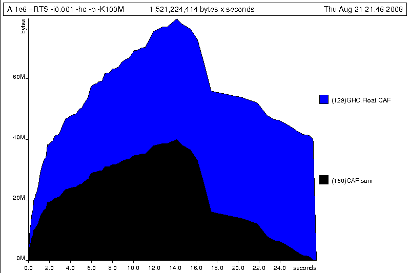
What does this graph tell us? For one, the program runs in two phases: spending
its first half allocating increasingly large amounts of memory, while summing
values, and the second half cleaning up those values. The initial allocation
also coincides with sum, doing some work, allocating a lot of
data. We get a slightly different presentation if we break down the allocation
by type, using -hy profiling:
$time ./A 1e6 +RTS -hy -p -K100M500000.5 ./A 1e6 +RTS -i0.001 -hy -p -K100M 34.96s user 0.22s system 99% cpu 35.237 total $ hp2ps -e8in -c A.hp
Which yields the following graph:
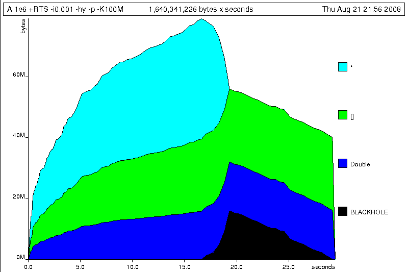
The most interesting things to notice here are large parts of the heap devoted
to values of list type (the [] band), and heap-allocated
Double values. There's also some heap allocated data of unknown
type (represented as data of type "*"). Finally, let's break it down by what
constructors are being allocated, using the -hd flag:
$time ./A 1e6 +RTS -hd -p -K100M$ time ./A 1e6 +RTS -i0.001 -hd -p -K100M 500000.5 ./A 1e6 +RTS -i0.001 -hd -p -K100M 27.85s user 0.31s system 99% cpu 28.222 total
Our final graphic reveals the full story of what is going on:
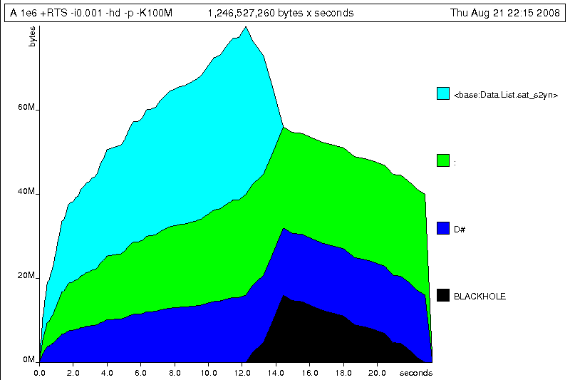
A lot of work is going into allocating list nodes containing double-precision
floating point values. Haskell lists are lazy, so the full million element
list is built up over time. Crucially, though, it is not being deallocated as it is
traversed, leading to increasingly large resident memory use. Finally, a bit
over halfway through the program run, the program finally finishes
summing the list, and starts calculating the length. If we look at the
original fragment for mean, we can see exactly why that memory
is being retained:
-- file: ch25/Fragment.hs
mean :: [Double] -> Double
mean xs = sum xs / fromIntegral (length xs)
At first we sum our list, which triggers the allocation of list nodes, but
we're unable to release the list nodes once we're done, as the entire list is
still needed by length. As soon as
sum is done though, and length
starts consuming the list, the garbage collector can chase it along,
deallocating the list nodes, until we're done. These two phases of evaluation
give two strikingly different phases of allocation and deallocation, and
point at exactly what we need to do: traverse the list only once, summing and
averaging it as we go.
Controlling evaluation
We have a number of options if we want to write our loop to traverse the list only once. For example, we can write the loop as a fold over the list, or via explicit recursion on the list structure. Sticking to the high level approaches, we'll try a fold first:
-- file: ch25/B.hs
mean :: [Double] -> Double
mean xs = s / fromIntegral n
  where
    (n, s)     = foldl k (0, 0) xs
    k (n, s) x = (n+1, s+x)
Now, instead of taking the sum of the list, and retaining the list until we can take its length, we left-fold over the list, accumulating the intermediate sum and length values in a pair (and we must left-fold, since a right-fold would take us to the end of the list and work backwards, which is exactly what we're trying to avoid).
The body of our loop is the k function, which takes the
intermediate loop state, and the current element, and returns a new state with
the length increased by one, and the sum increased by the current element. When
we run this, however, we get a stack overflow:
$ghc -O2 --make B.hs -fforce-recomp$time ./B 1e6Stack space overflow: current size 8388608 bytes. Use `+RTS -Ksize' to increase it. ./B 1e6 0.44s user 0.10s system 96% cpu 0.565 total
We traded wasted heap for wasted stack! In fact, if we increase the stack size
to the size of the heap in our previous implementation, with the
-K runtime flag, the program runs to completion, and has similar
allocation figures:
$ghc -O2 --make B.hs -prof -auto-all -caf-all -fforce-recomp[1 of 1] Compiling Main ( B.hs, B.o ) Linking B ...$time ./B 1e6 +RTS -i0.001 -hc -p -K100M500000.5 ./B 1e6 +RTS -i0.001 -hc -p -K100M 38.70s user 0.27s system 99% cpu 39.241 total
Generating the heap profile, we see all the allocation is now in mean:
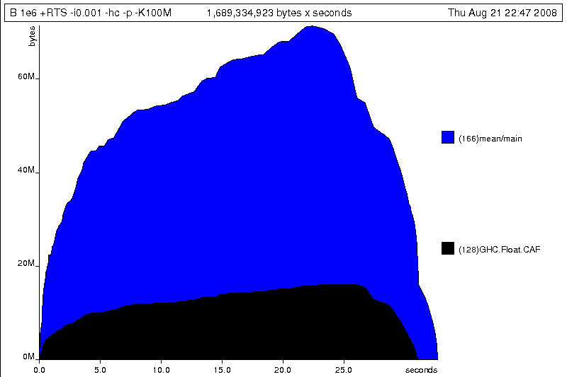
The question is: why are we building up more and more allocated state, when all we are doing is folding over the list? This, it turns out, is a classic space leak due to excessive laziness.
Strictness and tail recursion
The problem is that our left-fold, foldl, is too lazy.
What we want is a tail recursive loop, which can be implemented effectively
as a goto, with no state left on the stack. In this case
though, rather than fully reducing the tuple state at each step, a long chain
of thunks is being created, that only towards the end of the program is
evaluated. At no point do we demand reduction of the loop state, so the
compiler is unable to infer any strictness, and must reduce the value purely
lazily.
What we need to do is to tune the evaluation strategy slightly: lazily
unfolding the list, but strictly accumulating the fold state. The standard
approach here is to replace foldl with
foldl', from the Data.List module:
-- file: ch25/C.hs
mean :: [Double] -> Double
mean xs = s / fromIntegral n
  where
    (n, s)     = foldl' k (0, 0) xs
    k (n, s) x = (n+1, s+x)
However, if we run this implementation, we see we still haven't quite got it right:
$ghc -O2 --make C.hs[1 of 1] Compiling Main ( C.hs, C.o ) Linking C ...$time ./C 1e6Stack space overflow: current size 8388608 bytes. Use `+RTS -Ksize' to increase it. ./C 1e6 0.44s user 0.13s system 94% cpu 0.601 total
Still not strict enough! Our loop is continuing to accumulate unevaluated
state on the stack. The problem here is that foldl' is
only outermost strict:
-- file: ch25/Foldl.hs
foldl' :: (a -> b -> a) -> a -> [b] -> a
foldl' f z xs = lgo z xs
    where lgo z []     = z
          lgo z (x:xs) = let z' = f z x in z' `seq` lgo z' xs
This loop uses `seq` to reduce the accumulated state at
each step, but only to the outermost constructor on the loop state. That is,
seq reduces an expression to "weak head normal form". Evaluation
stops on the loop state once the first constructor is reached. In this case,
the outermost constructor is the tuple wrapper, (,), which
isn't deep enough. The problem is still the unevaluated numeric state inside
the tuple.
Adding strictness
There are a number of ways to make this function fully strict. We can, for example, add our own strictness hints to the internal state of the tuple, yielding a truly tail recursive loop:
-- file: ch25/D.hs
mean :: [Double] -> Double
mean xs = s / fromIntegral n
  where
    (n, s)     = foldl' k (0, 0) xs
    k (n, s) x = n `seq` s `seq` (n+1, s+x)
In this variant, we step inside the tuple state, and explicitly tell the compiler that each state component should be reduced, on each step. This gives us a version that does, at last, run in constant space:
$ghc -O2 D.hs --make[1 of 1] Compiling Main ( D.hs, D.o ) Linking D ...
If we run this, with allocation statistics enabled, we get the satisfying result:
$time ./D 1e6 +RTS -sstderr./D 1e6 +RTS -sstderr 500000.5 256,060,848 bytes allocated in the heap 43,928 bytes copied during GC (scavenged) 23,456 bytes copied during GC (not scavenged) 45,056 bytes maximum residency (1 sample(s)) 489 collections in generation 0 ( 0.00s) 1 collections in generation 1 ( 0.00s) 1 Mb total memory in use INIT time 0.00s ( 0.00s elapsed) MUT time 0.12s ( 0.13s elapsed) GC time 0.00s ( 0.00s elapsed) EXIT time 0.00s ( 0.00s elapsed) Total time 0.13s ( 0.13s elapsed) %GC time 2.6% (2.6% elapsed) Alloc rate 2,076,309,329 bytes per MUT second Productivity 97.4% of total user, 94.8% of total elapsed ./D 1e6 +RTS -sstderr 0.13s user 0.00s system 95% cpu 0.133 total
Unlike our first version, this program is 97.4% efficient, spending only 2.6% of its time doing garbage collection, and it runs in a constant 1 megabyte of space. It illustrates a nice balance between mixed strict and lazy evaluation, with the large list unfolded lazily, while we walk over it, strictly. The result is a program that runs in constant space, and does so quickly.
Normal form reduction
There are a number of other ways we could have addressed the strictness issue
here. For deep strictness, we can use the rnf function, part of
the parallel strategies library (along with using), which unlike
seq reduces to the fully evaluated "normal form" (hence its
name). Such a "deep seq" fold we can write as:
-- file: ch25/E.hs
import System.Environment
import Text.Printf
import Control.Parallel.Strategies

main = do
    [d] <- map read `fmap` getArgs
    printf "%f\n" (mean [1..d])

foldl'rnf :: NFData a => (a -> b -> a) -> a -> [b] -> a
foldl'rnf f z xs = lgo z xs
    where
        lgo z []     = z
        lgo z (x:xs) = lgo z' xs
            where
                z' = f z x `using` rnf

mean :: [Double] -> Double
mean xs = s / fromIntegral n
  where
    (n, s)     = foldl'rnf k (0, 0) xs
    k (n, s) x = (n+1, s+x) :: (Int, Double)
We change the implementation of foldl' to reduce the state to
normal form, using the rnf strategy. This also raises an issue
we avoided earlier: the type inferred for the loop accumulator state.
Previously, we relied on type defaulting to infer a numeric, integral type
for the length of the list in the accumulator, but switching to
rnf introduces the NFData class constraint, and we
can no longer rely on defaulting to set the length type.
Bang patterns
Perhaps the cheapest way, syntactically, to add required strictness to code that's excessively lazy is via "bang patterns" (whose name comes from pronunciation of the "!" character as "bang"), a language extension introduced with the following pragma:
-- file: ch25/F.hs
{-# LANGUAGE BangPatterns #-}
With bang patterns, we can hint at strictness on any binding form, making the
function strict in that variable. Much as explicit type annotations can
guide type inference, bang patterns can help guide strictness inference.
Bang patterns are a language extension, and are enabled with the
BangPatterns language pragma. We can now rewrite the loop state to be simply:
-- file: ch25/F.hs
mean :: [Double] -> Double
mean xs = s / fromIntegral n
  where
    (n, s)       = foldl' k (0, 0) xs
    k (!n, !s) x = (n+1, s+x)
The intermediate values in the loop state are now made strict, and the loop runs in constant space:
$ghc -O2 F.hs --make$time ./F 1e6 +RTS -sstderr./F 1e6 +RTS -sstderr 500000.5 256,060,848 bytes allocated in the heap 43,928 bytes copied during GC (scavenged) 23,456 bytes copied during GC (not scavenged) 45,056 bytes maximum residency (1 sample(s)) 489 collections in generation 0 ( 0.00s) 1 collections in generation 1 ( 0.00s) 1 Mb total memory in use INIT time 0.00s ( 0.00s elapsed) MUT time 0.14s ( 0.15s elapsed) GC time 0.00s ( 0.00s elapsed) EXIT time 0.00s ( 0.00s elapsed) Total time 0.14s ( 0.15s elapsed) %GC time 0.0% (2.3% elapsed) Alloc rate 1,786,599,833 bytes per MUT second Productivity 100.0% of total user, 94.6% of total elapsed ./F 1e6 +RTS -sstderr 0.14s user 0.01s system 96% cpu 0.155 total
In large projects, when we are investigating memory allocation hot spots, bang patterns are the cheapest way to speculatively modify the strictness properties of some code, as they're syntactically less invasive than other methods.
Strict data types
Strict data types are another effective way to provide strictness information to the compiler. By default, Haskell data types are lazy, but it is easy enough to add strictness information to the fields of a data type that then propagate through the program. We can declare a new strict pair type, for example:
-- file: ch25/G.hs
data Pair a b = Pair !a !b
This creates a pair type whose fields will always be kept in weak head normal form. We can now rewrite our loop as:
-- file: ch25/G.hs
mean :: [Double] -> Double
mean xs = s / fromIntegral n
  where
    Pair n s       = foldl' k (Pair 0 0) xs
    k (Pair n s) x = Pair (n+1) (s+x)
This implementation again has the same efficient, constant space behavior. At this point, to squeeze the last drops of performance out of this code, though, we have to dive a bit deeper.
Understanding Core
Besides looking at runtime profiling data, one sure way of determining exactly what your program is doing is to look at the final program source after the compiler is done optimizing it, particularly in the case of Haskell compilers, which can perform very aggressive transformations on the code. GHC uses what is humorously referred to as "a simple functional language", known as Core, as the compiler intermediate representation. It is essentially a subset of Haskell, augmented with unboxed data types (raw machine types, directly corresponding to primitive data types in languages like C), suitable for code generation. GHC optimizes Haskell by transformation, repeatedly rewriting the source into more and more efficient forms. The Core representation is the final functional version of your program, before translation to low level imperative code. In other words, Core has the final say, and if all-out performance is your goal, it is worth understanding.
To view the Core version of our Haskell program we compile with the
-ddump-simpl flag, or use the ghc-core tool, a
third-party utility that lets us view Core in a pager. So let's look at the
representation of our final fold using strict data types, in
Core form:
$ghc -O2 -ddump-simpl G.hs
A screenful of text is generated. If we look carefully at, we'll see a loop (here, cleaned up slightly for clarity):
lgo :: Integer -> [Double] -> Double# -> (# Integer, Double #)

lgo = \ n xs s ->
    case xs of
      []       -> (# n, D# s #);
      (:) x ys ->
        case plusInteger n 1 of
            n' -> case x of
                D# y -> lgo n' ys (+## s y)
This is the final version of our foldl', and tells us a lot
about the next steps for optimization. The fold itself has been entirely
inlined, yielding an explicit recursive loop over the list. The loop state,
our strict pair, has disappeared entirely, and the function now takes its
length and sum accumulators as direct arguments along with the list.
The sum of the list elements is represented with an unboxed
Double# value, a raw machine double kept in a
floating point register. This is ideal, as there will be no memory traffic
involved keeping the sum on the heap. However, the length of the list, since
we gave no explicit type annotation, has been inferred to be a heap-allocated
Integer, with requires a non-primitive plusInteger
to perform addition. If it is algorithmically sound to use a Int
instead, we can replace Integer with it, via a type annotation,
and GHC will then be able to use a raw machine Int# for the
length. We can hope for an improvement in time and space by ensuring both
loop components are unboxed, and kept in registers.
The base case of the loop, its end, yields an unboxed pair (a pair allocated
only in registers), storing the final length of the list, and the accumulated
sum. Notice that the return type is a heap-allocated Double
value, indicated by the D# constructor, which lifts a raw double
value onto the heap. Again this has implications for performance, as GHC
will need to check that there is sufficient heap space available before it can
allocate and return from the loop.
We can avoid this final heap check by having GHC return an unboxed
Double# value, which can be achieved by using a custom pair type
in the loop. In addition, GHC provides an optimiztion that unboxes the strict
fields of a data type, ensuring the fields of the new pair type will be
stored in registers. This optimization is turned on with
-funbox-strict-fields.
We can make both representation changes by replacing the polymorphic strict
pair type with one whose fields are fixed as Int and
Double:
-- file: ch25/H.hs
data Pair = Pair !Int !Double

mean :: [Double] -> Double
mean xs = s / fromIntegral n
  where
    Pair n s       = foldl' k (Pair 0 0) xs
    k (Pair n s) x = Pair (n+1) (s+x)
Compiling this with optimizations on, and -funbox-strict-fields -ddump-simpl,
we get a tighter inner loop in Core:
lgo :: Int# -> Double# -> [Double] -> (# Int#, Double# #)
lgo = \ n s xs ->
    case xs of
      []       -> (# n, s #)
      (:) x ys ->
        case x of
            D# y -> lgo (+# n 1) (+## s y) ys
Now the pair we use to represent the loop state is represented and returned as unboxed primitive types, and will be kept in registers. The final version now only allocates heap memory for the list nodes, as the list is lazily demanded. If we compile and run this tuned version, we can compare the allocation and time performance against our original program:
$time ./H 1e7 +RTS -sstderr./H 1e7 +RTS -sstderr 5000000.5 1,689,133,824 bytes allocated in the heap 284,432 bytes copied during GC (scavenged) 32 bytes copied during GC (not scavenged) 45,056 bytes maximum residency (1 sample(s)) 3222 collections in generation 0 ( 0.01s) 1 collections in generation 1 ( 0.00s) 1 Mb total memory in use INIT time 0.00s ( 0.00s elapsed) MUT time 0.63s ( 0.63s elapsed) GC time 0.01s ( 0.02s elapsed) EXIT time 0.00s ( 0.00s elapsed) Total time 0.64s ( 0.64s elapsed) %GC time 1.0% (2.4% elapsed) Alloc rate 2,667,227,478 bytes per MUT second Productivity 98.4% of total user, 98.2% of total elapsed ./H 1e7 +RTS -sstderr 0.64s user 0.00s system 99% cpu 0.644 total
While our original program, when operating on a list of 10 million elements, took more than a minute to run, and allocated more than 700 megabytes of memory, the final version, using a simple higher order fold, and a strict data type, runs in around half a second, and allocates a total of 1 megabyte. Quite an improvement!
The general rules we can learn from the profiling and optimization process are:
These simple strategies are enough to identify and squash untoward memory use issues, and when used wisely, can avoid them occurring in the first place.
Advanced techniques: fusion
The final bottleneck in our program is the lazy list itself. While we can
avoid allocating it all at once, there is still memory traffic each time
around the loop, as we demand the next cons cell in the list, allocate it to
the heap, operate on it, and continue. The list type is also polymorphic, so
the elements of the list will be represented as heap allocated
Double values.
What we'd like to do is eliminate the list entirely, keeping just the next element we need in a register. Perhaps surprisingly, GHC is able to transform the list program into a listless version, using an optimization known as deforestation, which refers to a general class of optimizations that involve eliminating intermediate data structures. Due to the absence of side effects, a Haskell compiler can be extremely aggressive when rearranging code, reordering and transforming wholesale at times. The specific deforestation optimization we will use here is stream fusion.
This optimization transforms recursive list generation and transformation
functions into non-recursive unfolds. When an
unfold appears next to a fold, the structure between
them is then eliminated entirely, yielding a single, tight loop, with no heap
allocation. The optimization isn't enabled by default, and it can radically
change the complexity of a piece of code, but is enabled by a number of data
structure libraries, which provide "rewrite rules", custom optimizations the
compiler applies to functions the library exports.
We'll use the uvector library, which provides a suite of
list-like operations that use stream fusion to remove intermediate data
structures. Rewriting our program to use streams is straightforward:
-- file: ch25/I.hs
import System.Environment
import Text.Printf
import Data.Array.Vector

main = do
    [d] <- map read `fmap` getArgs
    printf "%f\n" (mean (enumFromToFracU 1 d))

data Pair = Pair !Int !Double

mean :: UArr Double -> Double
mean xs = s / fromIntegral n
  where
    Pair n s       = foldlU k (Pair 0 0) xs
    k (Pair n s) x = Pair (n+1) (s+x)
After installing the uvector library, from Hackage, we can build
our program, with -O2 -funbox-strict-fields, and inspect the Core
that results:
fold :: Int# -> Double# -> Double# -> (# Int#, Double# #)
fold = \ n s t ->
    case >## t limit of {
      False -> fold (+# n 1) (+## s t) (+## t 1.0)
      True  -> (# n, s #)
This is really the optimal result! Our lists have been entirely fused away, yielding a tight loop where list generation is interleaved with accumulation, and all input and output variables are kept in registers. Running this, we see another improvement bump in performance, with runtime falling by another order of magnitude:
$ time ./I 1e7
5000000.5
./I 1e7  0.06s user 0.00s system 72% cpu 0.083 total
Tuning the generated assembly
Given that our Core is now optimal, the only step left to take this
program further is to look directly at the assembly. Of course, there
are only small gains left to make at this point. To view the generated
assembly, we can use a tool like ghc-core, or generate assembly
to standard output with the -ddump-asm flag to GHC. We have few
levers available to adjust the generated assembly, but we may choose between
the C and native code backends to GHC, and, if we choose the C backend, which
optimization flags to pass to GCC. Particularly with floating point code, it
is sometimes useful to compile via C, and enable specific high performance C
compiler optimizations.
For example, we can squeeze out the last drops of performance
from our final fused loop code by using -funbox-strict-fields -fvia-C -optc-O2, which
cuts the running time in half again (as the C compiler is able to optimize
away some redundant move instructions in the program's inner loop):
$ghc -fforce-recomp --make -O2 -funbox-strict-fields -fvia-C -optc-O2 I.hs[1 of 1] Compiling Main ( I.hs, I.o ) Linking I ...$time ./I 1e75000000.5 ./I 1e7 0.04s user 0.00s system 98% cpu 0.047 total
Inspecting the final x86_64 assembly (via -keep-tmp-files), we
see the generated loop contains only six instructions:
go:
  ucomisd     5(%rbx), %xmm6
  ja  .L31
  addsd       %xmm6, %xmm5
  addq        $1, %rsi
  addsd       .LC0(%rip), %xmm6
  jmp go
We've effectively massaged the program through multiple source-level optimizations, all the way to the final assembly. There's nowhere else to go from here. Optimising code to this level is very rarely necessary, of course, and typically only makes sense when writing low level libraries, or optimizing particularly important code, where all algorithm choices have already been determined. For day-to-day code, choosing better algorithms is always a more effective strategy, but it's useful to know we can optimize down to the metal if necessary.
Conclusions
In this chapter we've looked at a suite of tools and techniques you can use to track down and identify problematic areas of your code, along with a variety of conventions that can go a long way towards keeping your code lean and efficient. The goal is really to program in such a way that you have good knowledge of what your code is doing, at all levels from source, through the compiler, to the metal, and be able to focus in on particular levels when requirements demand.
By sticking to simple rules, choosing the right data structures, and avoiding the traps of the unwary, it is perfectly possible to reliably achieve high performance from your Haskell code, while being able to develop at a very high level. The result is a sweet balance of productivity and ruthless efficiency.
 Want to stay up to date? Subscribe to the comment feed for