Chapter 12. Barcode recognition
Table of Contents
- A little bit about barcodes
- Introducing arrays
- Encoding an EAN-13 barcode
- Constraints on our decoder
- Divide and conquer
- Turning a colour image into something tractable
- What have we done to our image?
- Finding matching digits
- Life without arrays or hash tables
- Turning digit soup into an answer
- Working with row data
- Pulling it all together
- A few comments on development style
In this chapter, we'll make use of the image parsing library we developed in Chapter 10, Code case study: parsing a binary data format to build a barcode recognition application. Given a picture of the back of a book taken with a camera phone, we could use this to extract its ISBN number.
A little bit about barcodes
The vast majority of packaged and mass-produced consumer goods sold have a barcode somewhere on them. Although there are dozens of barcode systems used across a variety specialised domains, consumer products typically use either UPC-A or EAN-13. UPC-A was developed in the United States, while EAN-13 is European in origin.
EAN-13 was developed after UPC-A, and is a superset of UPC-A. (In fact, UPC-A has been officially declared obsolete since 2005, though it's still widely used within the United States.) Any software or hardware that can understand EAN-13 barcodes will automatically handle UPC-A barcodes. This neatly reduces our descriptive problem to one standard.
As the name suggests, EAN-13 describes a 13-digit sequence, which is broken into four groups.
The first two digits describe the number system. This can either indicate the nationality of the manufacturer, or describe one of a few other categories, such as ISBN (book identifier) numbers.
The next five digits are a manufacturer ID, assigned by a country's numbering authority.
The five digits that follow are a product ID, assigned by the manufacturer. (Smaller manufacturers may have a longer manufacturer ID and shorter product ID, but they still add up to ten digits.)
The last digit is a check digit, allowing a scanner to validate the digit string it scans.
The only way in which an EAN-13 barcode differs from a UPC-A barcode is that the latter uses a single digit to represent its number system. EAN-13 barcodes retain UPC-A compatibility by setting the first number system digit to zero.
EAN-13 encoding
Before we worry about decoding an EAN-13 barcode, we need to understand how they are encoded. The system used by EAN-13 is a little involved. We start by computing the check digit, which is the last digit of a string.
-- file: ch12/Barcode.hs
checkDigit :: (Integral a) => [a] -> a
checkDigit ds = 10 - (sum products `mod` 10)
    where products = mapEveryOther (*3) (reverse ds)

mapEveryOther :: (a -> a) -> [a] -> [a]
mapEveryOther f = zipWith ($) (cycle [f,id])
This is one of those algorithms that is more
easily understood via the code than a verbal description. The
computation proceeds from the right of the string. Each
successive digit is either multiplied by three or left alone
(the cycle function repeats its input
list infinitely). The check digit is the difference between
their sum, modulo ten, and the number ten.
A barcode is a series of fixed-width bars, where black represents a binary “one” bit, and white a “zero”. A run of the same digits thus looks like a thicker bar.
The sequence of bits in a barcode is as follows.
The digits in the left and right groups have separate encodings. On the left, digits are encoded with parity bits. The parity bits encode the 13th digit of the barcode.
Introducing arrays
Before we continue, here are all of the imports that we will be using in the remainder of this chapter.
-- file: ch12/Barcode.hs
import Data.Array (Array(..), (!), bounds, elems, indices,
                   ixmap, listArray)

import Control.Applicative ((<$>))
import Control.Monad (forM_)
import Data.Char (digitToInt)
import Data.Ix (Ix(..))
import Data.List (foldl', group, sort, sortBy, tails)
import Data.Maybe (catMaybes, listToMaybe)
import Data.Ratio (Ratio)
import Data.Word (Word8)
import System.Environment (getArgs)
import qualified Data.ByteString.Lazy.Char8 as L
import qualified Data.Map as M

import Parse                    -- from chapter 11
The barcode encoding process can largely be table-driven, in which we use small tables of bit patterns to decide how to encode each digit. Haskell's bread-and-butter data types, lists and tuples, are not well suited to use for tables whose elements may be accessed randomly. A list has to be traversed linearly to reach the kth element. A tuple doesn't have this problem, but Haskell's type system makes it difficult to write a function that takes a tuple and an element offset and returns the element at that offset within the tuple. (We'll explore why in the exercises below.)
The usual data type for constant-time random access is of course the array. Haskell provides several array data types. We'll thus represent our encoding tables as arrays of strings.
The simplest array type is in the Data.Array
module, which we're using here. This presents arrays that can
contain values of any Haskell type. Like other common Haskell
types, these arrays are immutable. An immutable array is
populated with values just once, when it is created. Its
contents cannot subsequently be modified. (The standard
libraries also provide other array types, some of which are
mutable, but we won't cover those for a while.)
-- file: ch12/Barcode.hs
leftOddList = ["0001101", "0011001", "0010011", "0111101", "0100011",
               "0110001", "0101111", "0111011", "0110111", "0001011"]

rightList = map complement <$> leftOddList
    where complement '0' = '1'
          complement '1' = '0'

leftEvenList = map reverse rightList

parityList = ["111111", "110100", "110010", "110001", "101100",
              "100110", "100011", "101010", "101001", "100101"]

listToArray :: [a] -> Array Int a
listToArray xs = listArray (0,l-1) xs
    where l = length xs

leftOddCodes, leftEvenCodes, rightCodes, parityCodes :: Array Int String

leftOddCodes = listToArray leftOddList
leftEvenCodes = listToArray leftEvenList
rightCodes = listToArray rightList
parityCodes = listToArray parityList
The Data.Array module's
listArray function populates an array from
a list. It takes as its first parameter the bounds of the array
to create; the second is the values with which to populate
it.
An unusual feature of the Array type is that its type is parameterised over both the data it contains and the index type. For example, the type of a one-dimensional array of String is Array Int String, but a two-dimensional array would have the type Array (Int,Int) String.
ghci>:m +Data.Arrayghci>:type listArraylistArray :: (Ix i) => (i, i) -> [e] -> Array i e
We can construct an array easily.
ghci>listArray (0,2) "foo"array (0,2) [(0,'f'),(1,'o'),(2,'o')]
Notice that we have to specify the lower and upper bounds of the array. These bounds are inclusive, so an array from 0 to 2 has elements 0, 1, and 2.
ghci>listArray (0,3) [True,False,False,True,False]array (0,3) [(0,True),(1,False),(2,False),(3,True)]ghci>listArray (0,10) "too short"array (0,10) [(0,'t'),(1,'o'),(2,'o'),(3,' '),(4,'s'),(5,'h'),(6,'o'),(7,'r'),(8,'t'),(9,*** Exception: (Array.!): undefined array element
Once an array is constructed, we can use the
(!) operator to access its elements by
index.
ghci>let a = listArray (0,14) ['a'..]ghci>a ! 2'c'ghci>a ! 100*** Exception: Error in array index
Since the array construction function lets us specify the bounds of an array, we don't have to use the zero-based array indexing familiar to C programmers. We can choose whatever bounds are convenient for our purposes.
ghci>let a = listArray (-9,5) ['a'..]ghci>a ! (-2)'h'
The index type can be any member of the Ix type. This lets us use, for example, Char as the index type.
ghci>let a = listArray ('a', 'h') [97..]ghci>a ! 'e'101
To create a higher-dimensioned array, we use a tuple of Ix instances as the index type. The Prelude makes tuples of up to five elements members of the Ix class. To illustrate, here's a small three-dimensional array.
ghci>let a = listArray ((0,0,0), (9,9,9)) [0..]ghci>a ! (4,3,7)437
Arrays and laziness
The list that we use to populate the array must contain at least as many elements as are in the array. If we do not provide enough elements, we'll get an error at runtime. When the error will occur depends on the nature of the array.
Here, we are using an array type that is non-strict in its elements. If we provide a list of three values to an array that we specify as containing more than three elements, the remaining elements will undefined. We will not get an error unless we access an element beyond the third.
ghci>let a = listArray (0,5) "bar"ghci>a ! 2'r'ghci>a ! 4*** Exception: (Array.!): undefined array element
Haskell also provides strict arrays, which behave differently. We will discuss the tradeoffs between the two kinds of array much later, in the section called “Unboxing, lifting, and bottom”.
Folding over arrays
The bounds function returns a tuple
describing the bounds that we used to create the array. The
indices function returns a list of every
index. We can use these to define some useful folds, since
the Data.Array module doesn't define any fold
functions itself.
-- file: ch12/Barcode.hs
-- | Strict left fold, similar to foldl' on lists.
foldA :: Ix k => (a -> b -> a) -> a -> Array k b -> a
foldA f s a = go s (indices a)
    where go s (j:js) = let s' = f s (a ! j)
                        in s' `seq` go s' js
          go s _ = s

-- | Strict left fold using the first element of the array as its
-- starting value, similar to foldl1 on lists.
foldA1 :: Ix k => (a -> a -> a) -> Array k a -> a
foldA1 f a = foldA f (a ! fst (bounds a)) a
You might wonder why the array modules don't already provide such useful things as folding functions. There are some obvious correspondences between a one-dimensional array and a list. For instance, there are only two natural ways in which we can fold sequentially: left-to-right and right-to-left. Additionally, we can only fold over one element at a time.
This does not translate even to two-dimensional arrays. First of all, there are several kinds of fold that make sense. We might still want to fold over single elements, but we now have the possibility of folding over rows or columns, too. On top of this, for element-at-a-time folding, there are no longer just two sequences for traversal.
In other words, for two-dimensional arrays, there are enough permutations of possibly useful behaviour that there aren't many compelling reasons to choose a handful for a standard library. This problem is only compounded for higher dimensions, so it's best to let developers write folds that suit the needs of their applications. As we can see from our examples above, this is not hard to do.
Modifying array elements
While there exist “modification” functions
for immutable arrays, they are not very practical. For
example, the accum function takes an
array and a list of (index, value) pairs, and
returns a new array with the values at the given indices
replaced.
Since arrays are immutable, modifying even one element requires copying the entire array. This quickly becomes prohibitively expensive on arrays of even modest size.
Another array type, DiffArray in
the Data.Array.Diff module, attempts to offset
the cost of small modifications by storing deltas between
successive versions of an array. Unfortunately, it is not
implemented efficiently at the time we are writing this book,
and is currently too slow to be of practical use.
![[Note]](/support/figs/note.png) | Don't lose hope |
|---|---|
It is in fact possible to modify an array efficiently in Haskell, using the ST monad. This is a subject that we will return to later, in Chapter 26, Advanced library design: building a Bloom filter. |
Exercises
Let's briefly explore the suitability of tuples as stand-ins for arrays.
Encoding an EAN-13 barcode
Even though our goal is to
decode a barcode, it's useful to have an
encoder for reference. This will allow us to, for example,
ensure that our code is correct by checking that the output of
decode . encode the same as its input.
-- file: ch12/Barcode.hs
encodeEAN13 :: String -> String
encodeEAN13 = concat . encodeDigits . map digitToInt

-- | This function computes the check digit; don't pass one in.
encodeDigits :: [Int] -> [String]
encodeDigits s@(first:rest) =
    outerGuard : lefties ++ centerGuard : righties ++ [outerGuard]
  where (left, right) = splitAt 5 rest
        lefties = zipWith leftEncode (parityCodes ! first) left
        righties = map rightEncode (right ++ [checkDigit s])

leftEncode :: Char -> Int -> String
leftEncode '1' = (leftOddCodes !)
leftEncode '0' = (leftEvenCodes !)

rightEncode :: Int -> String
rightEncode = (rightCodes !)

outerGuard = "101"
centerGuard = "01010"
The string to encode is twelve digits long, with
encodeDigits adding a thirteenth check
digit.
The barcode is encoded as two groups of six digits, with a guard sequence in the middle and “outside” sequences on either side. But if we have two groups of six digits, what happened to the missing digit?
Each digit in the left group is encoded using either odd or even parity, with the parity chosen based on the bits of the first digit in the string. If a bit of the first digit is zero, the corresponding digit in the left group is encoded with even parity. A one bit causes the digit to be encoded with odd parity. This encoding is an elegant hack, chosen to make EAN-13 barcodes backwards compatible with the older UPC-A standard.
Constraints on our decoder
Before we talk about decoding, let's set a few practical limits on what kinds of barcode image we can work with.
Phone cameras and webcams generally output JPEG images, but writing a JPEG decoder would take us several chapters. We'll simplify our parsing problem by handling the netpbm file format. We will use the parsing combinators we developed earlier, in Chapter 10, Code case study: parsing a binary data format.
We'd like to deal with real images from the kinds of cheap, fixed-focus cameras that come with low-end cell phones. These images tend to be out of focus, noisy, low in contrast, and of poor resolution. Fortunately, it's not hard to write code that can handle noisy, defocused VGA-resolution (640x480) images with terrible contrast ratios. We've verified that the code in this chapter captures barcodes from real books, using pictures taken by authentically mediocre cameras.
We will avoid any image processing heroics, because that's another chapter-consuming subject. We won't correct perspective. Neither will we sharpen images taken from too near to the subject, which causes narrow bars to fade out; or from too far, which causes adjacent bars to blur together.
Divide and conquer
Our task is to take a camera image and extract a valid barcode from it. Given such a nonspecific description, it can be hard to see how to make progress. However, we can break the big problem into a series of subproblems, each of which is self-contained and more tractable.
Many of these subproblems can be further divided, as we'll see.
You might wonder how closely this approach of subdivision mirrors the actual work we did when writing the code that we present in this chapter. The answer is that we're far from image processing gurus, and when we started on this chapter we didn't know exactly what our solution was going to look like.
We made some early educated guesses as to what a reasonable solution might look like, and came up with the list of subtasks above. We were then able to start tackling those parts that we knew how to solve, using our spare time to think about the bits that we had no prior experience with. We certainly didn't have a pre-existing algorithm or master plan in mind.
Dividing the problem up like this helped us in two ways. By making progress on familiar ground, we had the psychological advantage of starting to solve the problem, even when we didn't really know where we were going. And as we started to work on a particular subproblem, we found ourselves able to further subdivide it into tasks of varying familiarity. We continued to focus on easier components, deferring ones we hadn't thought about in enough detail yet, and jumping from one element of the master list above to another. Eventually, we ran out of problems that were both unfamiliar and unsolved, and we had a complete idea of our eventual solution.
Turning a colour image into something tractable
Since we want to work with barcodes, which are sequences of black and white stripes, and we want to write a simple decoder, an easy representation to work with will be a monochrome image, in which each pixel is either black or white.
Parsing a colour image
As we mentioned earlier, we'll work with netpbm images. The netpbm colour image format is only slightly more complicated than the greyscale image format that we parsed in Chapter 10, Code case study: parsing a binary data format. The identifying string in a header is “P6”, with the rest of the header layout identical to the greyscale format. In the body of an image, each pixel is represented as three bytes, one each for red, green and blue.
We'll represent the image data as a two-dimensional array of pixels. We're using arrays here purely to gain experience with them. For this application, we could just as well use a list of lists. The only advantage of an array here is slight: we can efficiently extract a row.
-- file: ch12/Barcode.hs
type Pixel = Word8
type RGB = (Pixel, Pixel, Pixel)

type Pixmap = Array (Int,Int) RGB
We provide a few type synonyms to make our type signatures more readable.
Since Haskell gives us considerable freedom in how we lay
out an array, we must choose a representation. We'll play
safe and follow a popular convention: indices begin at zero.
We don't need to store the dimensions of the image explicitly,
since we can extract them using the
bounds function.
The actual parser is mercifully short, thanks to the combinators we developed in Chapter 10, Code case study: parsing a binary data format.
-- file: ch12/Barcode.hs
parseRawPPM :: Parse Pixmap
parseRawPPM =
    parseWhileWith w2c (/= '\n') ==> \header -> skipSpaces ==>&
    assert (header == "P6") "invalid raw header" ==>&
    parseNat ==> \width -> skipSpaces ==>&
    parseNat ==> \height -> skipSpaces ==>&
    parseNat ==> \maxValue ->
    assert (maxValue == 255) "max value out of spec" ==>&
    parseByte ==>&
    parseTimes (width * height) parseRGB ==> \pxs ->
    identity (listArray ((0,0),(width-1,height-1)) pxs)

parseRGB :: Parse RGB
parseRGB = parseByte ==> \r ->
           parseByte ==> \g ->
           parseByte ==> \b ->
           identity (r,g,b)

parseTimes :: Int -> Parse a -> Parse [a]
parseTimes 0 _ = identity []
parseTimes n p = p ==> \x -> (x:) <$> parseTimes (n-1) p
The only function of note above is
parseTimes, which calls another parser a
given number of times, building up a list of results.
Greyscale conversion
Now that we have a colour image in hand, we need to convert the colour data into monochrome. An intermediate step is to convert the data to greyscale. There's a simple, widely used formula[29] for converting an RGB image into a greyscale image, based on the perceived brightness of each colour channel.
-- file: ch12/Barcode.hs
luminance :: (Pixel, Pixel, Pixel) -> Pixel
luminance (r,g,b) = round (r' * 0.30 + g' * 0.59 + b' * 0.11)
    where r' = fromIntegral r
          g' = fromIntegral g
          b' = fromIntegral b
Haskell arrays are members of the Functor
typeclass, so we can simply use fmap to
turn an entire image, or a single scanline, from colour into
greyscale.
-- file: ch12/Barcode.hs
type Greymap = Array (Int,Int) Pixel

pixmapToGreymap :: Pixmap -> Greymap
pixmapToGreymap = fmap luminance
This pixmapToGreymap function is just
for illustration. Since we'll only be checking a few rows of
an image for possible barcodes, there's no reason to do the
extra work of converting data we'll never subsequently
use.
Greyscale to binary, and type safety
Our next subproblem is to convert the greyscale image into a two-valued image, where each pixel is either on or off.
In an image processing application, where we're juggling lots of numbers, it would be easy to reuse the same numeric type for several different purposes. For example, we could use the Pixel type to represent on/off states, using the convention that the digit one represents a bit that's “on”, and zero “off”.
However, reusing types for multiple purposes in this way quickly leads to potential confusion. To see whether a particular “Pixel” is a number or an on/off value, we can no longer simply glance at a type signature. We could easily use a value containing “the wrong kind of number” in some context, and the compiler won't catch it because the types work out.
We could try to work around this by introducing a type alias. In the same way that we declared Pixel to be a synonym of Word8, we could declare a Bit type as a synonym of Pixel. While this might help readability, type synonyms still don't make the compiler do any useful work on our behalf.
The compiler would treat Pixel and Bit as exactly the same type, so it could not catch a mistake such as using a Pixel value of 253 in a function that expects Bit values of zero or one.
If we define the monochrome type ourselves, the compiler will prevent us from accidentally mixing our types up like this.
-- file: ch12/Barcode.hs
data Bit = Zero | One
           deriving (Eq, Show)

threshold :: (Ix k, Integral a) => Double -> Array k a -> Array k Bit
threshold n a = binary <$> a
    where binary i | i < pivot  = Zero
                   | otherwise  = One
          pivot    = round $ least + (greatest - least) * n
          least    = fromIntegral $ choose (<) a
          greatest = fromIntegral $ choose (>) a
          choose f = foldA1 $ \x y -> if f x y then x else y
Our threshold function computes the
minimum and maximum values in its input array. It takes these
and a threshold valued between zero and one, and computes a
“pivot” value. Then for each value in the array,
if that value is less than the pivot, the result is
Zero, otherwise One. Notice that we
use one of the folding functions that we wrote in the section called “Folding over arrays”.
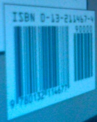
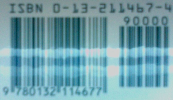
What have we done to our image?
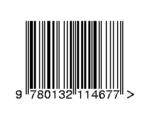
Let's step back for a moment and consider what we've done to our image when we converted it from colour to monochrome. Here's an image captured from a VGA-resolution camera. All we've done is crop it down to the barcode.
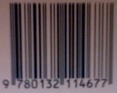
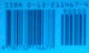
The encoded digit string, 9780132114677, is printed below the barcode. The left group encodes the digits 780132, with 9 encoded in their parity. The right group encodes the digits 114677, where the final 7 is the check digit. Here's a clean encoding of this barcode, from one of the many web sites that offer barcode image generation for free.
We've chosen a row from the captured image, and stretched it out vertically to make it easier to see. We've superimposed this on top of the perfect image, and stretched it out so that the two are aligned.
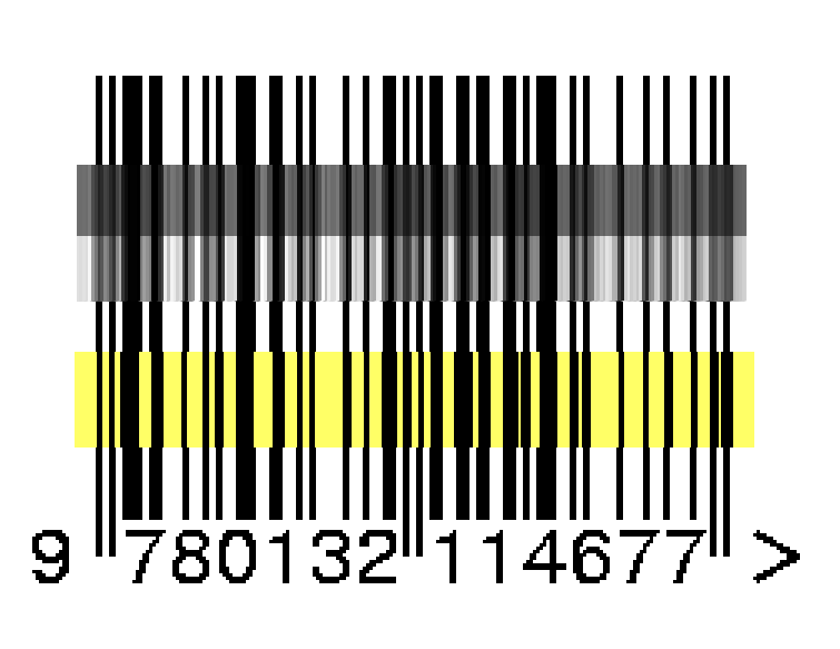
The luminance-converted row from the photo is in the dark grey band. It is low in contrast and poor in quality, with plenty of blurring and noise. The paler band is the same row with the contrast adjusted.
Somewhat below these two bands is another: this shows the effect of thresholding the luminance-converted row. Notice that some bars have gotten thicker, others thinner, and many bars have moved a little to the left or right.
Clearly, any attempt to find exact matches in an image with problems like these is not going to succeed very often. We must write code that's robust in the face of bars that are too thick, too thin, or not exactly where they're supposed to be. The widths of our bars will depend on how far our book was from the camera, so we can't make any assumptions about widths, either.
Finding matching digits
Our first problem is to find the digits that might be encoded at a given position. For the next while, we'll make a few simplifying assumptions. The first is that we're working with a single row. The second is that we know exactly where in a row the left edge of a barcode begins.
Run length encoding
How can we overcome the problem of not even knowing how thick our bars are? The answer is to run length encode our image data.
-- file: ch12/Barcode.hs
type Run = Int
type RunLength a = [(Run, a)]

runLength :: Eq a => [a] -> RunLength a
runLength = map rle . group
    where rle xs = (length xs, head xs)
The group function takes sequences of
identical elements in a list, and groups them into
sublists.
ghci>group [1,1,2,3,3,3,3][[1,1],[2],[3,3,3,3]]
Our runLength function represents
each group as a pair of its length and first element.
ghci>let bits = [0,0,1,1,0,0,1,1,0,0,0,0,0,0,1,1,1,1,0,0,0,0]ghci>runLength bitsLoading package array-0.1.0.0 ... linking ... done. Loading package containers-0.1.0.1 ... linking ... done. Loading package bytestring-0.9.0.1 ... linking ... done. [(2,0),(2,1),(2,0),(2,1),(6,0),(4,1),(4,0)]
Since the data we're run length encoding are just ones and zeros, the encoded numbers will simply alternate between one and zero. We can throw the encoded values away without losing any useful information, keeping only the length of each run.
-- file: ch12/Barcode.hs
runLengths :: Eq a => [a] -> [Run]
runLengths = map fst . runLength
ghci>runLengths bits[2,2,2,2,6,4,4]
The bit patterns above aren't random; they're the left
outer guard and first encoded digit of a row from our captured
image. If we drop the guard bars, we're left with the run
lengths [2,6,4,4]. How do we find matches
for these in the encoding tables we wrote in the section called “Introducing arrays”?
Scaling run lengths, and finding approximate matches
One possible approach is to scale the run lengths so that they sum to one. We'll use the Ratio Int type instead of the usual Double to manage these scaled values, as Ratios print out more readably in ghci. This makes interactive debugging and development much easier.
-- file: ch12/Barcode.hs
type Score = Ratio Int

scaleToOne :: [Run] -> [Score]
scaleToOne xs = map divide xs
    where divide d = fromIntegral d / divisor
          divisor = fromIntegral (sum xs)
-- A more compact alternative that "knows" we're using Ratio Int:
-- scaleToOne xs = map (% sum xs) xs

type ScoreTable = [[Score]]

-- "SRL" means "scaled run length".
asSRL :: [String] -> ScoreTable
asSRL = map (scaleToOne . runLengths)

leftOddSRL = asSRL leftOddList
leftEvenSRL = asSRL leftEvenList
rightSRL = asSRL rightList
paritySRL = asSRL parityList
We use the Score type synonym so that most of our code won't have to care what the underlying type is. Once we're done developing our code and poking around with ghci, we could, if we wish, go back and turn the “Score” type synonym into Doubles, without changing any code.
We can use scaleToOne to scale a
sequence of digits that we're searching for. We've now
corrected for variations in bar widths due to distance, as
there should be a pretty close match between an entry in a
scaled run length encoding table and a run length sequence
pulled from an image.
The next question is how we turn the intuitive idea of “pretty close” into a measure of “close enough”. Given two scaled run length sequences, we can calculate an approximate “distance” between them as follows.
-- file: ch12/Barcode.hs
distance :: [Score] -> [Score] -> Score
distance a b = sum . map abs $ zipWith (-) a b
An exact match will give a distance of zero, with weaker matches resulting in larger distances.
ghci>let group = scaleToOne [2,6,4,4]ghci>distance group (head leftEvenSRL)13%28ghci>distance group (head leftOddSRL)17%28
Given a scaled run length table, we choose the best few matches in that table for a given input sequence.
-- file: ch12/Barcode.hs
bestScores :: ScoreTable -> [Run] -> [(Score, Digit)]
bestScores srl ps = take 3 . sort $ scores
    where scores = zip [distance d (scaleToOne ps) | d <- srl] digits
          digits = [0..9]
List comprehensions
The new notation that we introduced in the previous example is an example of a list comprehension, which creates a list from one or more other lists.
ghci>[ (a,b) | a <- [1,2], b <- "abc" ][(1,'a'),(1,'b'),(1,'c'),(2,'a'),(2,'b'),(2,'c')]
The expression on the left of the vertical bar is
evaluated for each combination of generator
expressions on the right. A generator expression
binds a variable on the left of a <- to an element of
the list on the right. As the example above shows, the
combinations of generators are evaluated in depth first order:
for the first element of the first list, we evaluate every
element of the second, and so on.
In addition to generators, we can also specify guards on
the right of a list comprehension. A guard is a
Bool expression. If it evaluates to
False, that element is skipped over.
ghci>[ (a,b) | a <- [1..6], b <- [5..7], even (a + b ^ 2) ][(1,5),(1,7),(2,6),(3,5),(3,7),(4,6),(5,5),(5,7),(6,6)]
We can also bind local variables using a let
expression.
ghci>let vowel = (`elem` "aeiou")ghci>[ x | a <- "etaoin", b <- "shrdlu", let x = [a,b], all vowel x ]["eu","au","ou","iu"]
If a pattern match fails in a generator expression, no error occurs. Instead, that list element is skipped.
ghci>[ a | (3,a) <- [(1,'y'),(3,'e'),(5,'p')] ]"e"
List comprehensions are powerful and concise. As a result, they can be difficult to read. When used with care, they can make our code easier to follow.
-- file: ch12/Barcode.hs
-- our original
zip [distance d (scaleToOne ps) | d <- srl] digits

-- the same expression, expressed without a list comprehension
zip (map (flip distance (scaleToOne ps)) srl) digits

-- the same expression, written entirely as a list comprehension
[(distance d (scaleToOne ps), n) | d <- srl, n <- digits]
Remembering a match's parity
For each match in the left group, we have to remember whether we found it in the even parity table or the odd table.
-- file: ch12/Barcode.hs
data Parity a = Even a | Odd a | None a
                deriving (Show)

fromParity :: Parity a -> a
fromParity (Even a) = a
fromParity (Odd a) = a
fromParity (None a) = a

parityMap :: (a -> b) -> Parity a -> Parity b
parityMap f (Even a) = Even (f a)
parityMap f (Odd a) = Odd (f a)
parityMap f (None a) = None (f a)

instance Functor Parity where
    fmap = parityMap
We wrap a value in the parity with which it was
encoded, and making it a Functor instance so that
we can easily manipulate parity-encoded values.
We would like to be able to sort parity-encoded
values based on the values they contain. The
Data.Function module provides a lovely combinator
that we can use for this, named
on.
-- file: ch12/Barcode.hs
on :: (a -> a -> b) -> (c -> a) -> c -> c -> b
on f g x y = g x `f` g y

compareWithoutParity = compare `on` fromParity
In case it's unclear, try thinking of
on as a function of two arguments,
f and g, which returns a
function of two arguments, x and
y. It applies g to
x and to y, then
f on the two results (hence the name
on).
Wrapping a match in a parity value is straightforward.
-- file: ch12/Barcode.hs
type Digit = Word8

bestLeft :: [Run] -> [Parity (Score, Digit)]
bestLeft ps = sortBy compareWithoutParity
              ((map Odd (bestScores leftOddSRL ps)) ++
               (map Even (bestScores leftEvenSRL ps)))

bestRight :: [Run] -> [Parity (Score, Digit)]
bestRight = map None . bestScores rightSRL
Once we have the best left-hand matches from the even and odd tables, we sort them based only on the quality of each match.
Another kind of laziness, of the keyboarding variety
In our definition of the Parity type, we could have used Haskell's record syntax to avoid the need to write a fromParity function. In other words, we could have written it as follows.
-- file: ch12/Barcode.hs
data AltParity a = AltEven {fromAltParity :: a}
                 | AltOdd  {fromAltParity :: a}
                 | AltNone {fromAltParity :: a}
                   deriving (Show)
Why did we not do this? The answer is slightly shameful, and has to do with interactive debugging in ghci. When we tell GHC to automatically derive a Show instance for a type, it produces different code depending on whether or not we declare the type with record syntax.
ghci>show $ Even 1"Even 1"ghci>show $ AltEven 1"AltEven {fromAltParity = 1}"ghci>length . show $ Even 16ghci>length . show $ AltEven 127
The Show instance for the variant that uses record syntax is considerably more verbose. This creates much more noise that we must scan through when we're trying to read, say, a list of parity-encoded values output by ghci.
Of course we could write our own, less noisy, Show instance. It's simply less effort to avoid record syntax and write our own fromParity function instead, letting GHC derive a more terse Show instance for us. This isn't an especially satisfying rationale, but programmer laziness can lead in odd directions at times.
Chunking a list
A common aspect of working with lists is needing to “chunk” them. For example, each digit in a barcode is encoded using a run of four digits. We can turn the flat list that represents a row into a list of four-element lists as follows.
-- file: ch12/Barcode.hs
chunkWith :: ([a] -> ([a], [a])) -> [a] -> [[a]]
chunkWith _ [] = []
chunkWith f xs = let (h, t) = f xs
                 in h : chunkWith f t

chunksOf :: Int -> [a] -> [[a]]
chunksOf n = chunkWith (splitAt n)
It's somewhat rare that we need to write generic
list manipulation functions like this. Often, a
glance through the Data.List module will find us
a function that does exactly, or close enough to, what we
need.
Generating a list of candidate digits
With our small army of helper functions deployed, the
function that generates lists of candidate matches for each
digit group is easy to write. First of all, we take care of a
few early checks to determine whether matching even makes
sense. A list of runs must start on a black
(Zero) bar, and contain enough bars. Here are
the first few equations of our function.
-- file: ch12/Barcode.hs
candidateDigits :: RunLength Bit -> [[Parity Digit]]
candidateDigits ((_, One):_) = []
candidateDigits rle | length rle < 59 = []
If any application of
bestLeft or
bestRight results in an empty list, we
can't possibly have a match. Otherwise, we throw away the
scores, and return a list of lists of parity-encoded candidate
digits. The outer list is twelve elements long, one per digit
in the barcode. The digits in each sublist are ordered by
match quality.
Here is the remainder of the definition of our function.
-- file: ch12/Barcode.hs
candidateDigits rle
    | any null match = []
    | otherwise      = map (map (fmap snd)) match
  where match = map bestLeft left ++ map bestRight right
        left = chunksOf 4 . take 24 . drop 3 $ runLengths
        right = chunksOf 4 . take 24 . drop 32 $ runLengths
        runLengths = map fst rle
Let's take a glance at the candidate digits chosen for each group of bars, from a row taken from the image above.
ghci>:type inputinput :: [(Run, Bit)]ghci>take 7 input[(2,Zero),(2,One),(2,Zero),(2,One),(6,Zero),(4,One),(4,Zero)]ghci>mapM_ print $ candidateDigits input[Even 1,Even 5,Odd 7,Odd 1,Even 2,Odd 5] [Even 8,Even 7,Odd 1,Odd 2,Odd 0,Even 6] [Even 0,Even 1,Odd 8,Odd 2,Odd 4,Even 9] [Odd 1,Odd 0,Even 8,Odd 2,Even 2,Even 4] [Even 3,Odd 4,Odd 5,Even 7,Even 0,Odd 2] [Odd 2,Odd 4,Even 7,Even 0,Odd 1,Even 1] [None 1,None 5,None 0] [None 1,None 5,None 2] [None 4,None 5,None 2] [None 6,None 8,None 2] [None 7,None 8,None 3] [None 7,None 3,None 8]
Life without arrays or hash tables
In an imperative language, the array is as much a “bread and butter” type as a list or tuple in Haskell. We take it for granted that an array in an imperative language is usually mutable; we can change an element of an array whenever it suits us.
As we mentioned in the section called “Modifying array elements”, Haskell arrays are not mutable. This means that to “modify” a single array element, a copy of the entire array is made, with that single element set to its new value. Clearly, this approach is not a winner for performance.
The mutable array is a building block for another ubiquitous imperative data structure, the hash table. In the typical implementation, an array acts as the “spine” of the table, with each element containing a list of elements. To add an element to a hash table, we hash the element to find the array offset, and modify the list at that offset to add the element to it.
If arrays aren't mutable, to updating a hash table, we must create a new one. We copy the array, putting a new list at the offset indicated by the element's hash. We don't need to copy the lists at other offsets, but we've already dealt performance a fatal blow simply by having to copy the spine.
At a single stroke, then, immutable arrays have eliminated two canonical imperative data structures from our toolbox. Arrays are somewhat less useful in pure Haskell code than in many other languages. Still, many array codes only update an array during a build phase, and subsequently use it in a read-only manner.
A forest of solutions
This is not the calamitous situation that it might seem, though. Arrays and hash tables are often used as collections indexed by a key, and in Haskell we use trees for this purpose.
Implementing a naive tree type is particularly easy in Haskell. Beyond that, more useful tree types are also unusually easy to implement. Self-balancing structures, such as red-black trees, have struck fear into generations of undergraduate computer science students, because the balancing algorithms are notoriously hard to get right.
Haskell's combination of algebraic data types, pattern matching, and guards reduce even the hairiest of balancing operations to a few lines of code. We'll bite back our enthusiasm for building trees, however, and focus on why they're particularly useful in a pure functional language.
The attraction of a tree to a functional programmer is cheap modification. We don't break the immutability rule: trees are immutable just like everything else. However, when we modify a tree, creating a new tree, we can share most of the structure of the tree between the old and new versions. For example, in a tree containing 10,000 nodes, we might expect that the old and new versions will share about 9,985 elements when we add or remove one. In other words, the number of elements modified per update depends on the height of the tree, or the logarithm of the size of the tree.
Haskell's standard libraries provide two collection types
that are implemented using balanced trees behind the scenes:
Data.Map for key/value pairs, and
Data.Set for sets of values. As we'll be using
Data.Map in the sections that follow, we'll give
a quick introduction to it below. Data.Set is
sufficiently similar that you should be able to pick it up
quickly.
A brief introduction to maps
The Data.Map module provides a
parameterised type, Map k a, that maps from a key
type k to a value type a. Although it is internally a
size-balanced binary tree, the implementation is not visible
to us.
Map is strict in its keys, but non-strict in its values. In other words, the spine, or structure, of the map is always kept up to date, but values in the map aren't evaluated unless we force them to be.
It is very important to remember this, as Map's laziness over values is a frequent source of space leaks among coders who are not expecting it.
Because the Data.Map module
contains a number of names that clash with Prelude names, it's
usually imported in qualified form. Earlier in this chapter,
we imported it using the prefix M.
Type constraints
The Map type doesn't place any explicit
constraints on its key type, but most of the module's useful
functions require that keys be instances of
Ord. This is noteworthy, as it's an example of
a common design pattern in Haskell code: type constraints
are pushed out to where they're actually needed, not
necessarily applied at the point where they'd result in the
least fingertyping for a library's author.
Neither the Map type nor any functions in the module constrain the types that can be used as values.
Partial application awkwardness
For some reason, the type signatures of the functions in
Data.Map are not generally friendly to partial
application. The map parameter always comes last, whereas it
would be easier to partially apply if it were first. As a
result, code that uses partially applied map functions
almost always contains adapter functions to fiddle with
argument ordering.
Getting started with the API
The Data.Map module has a large
“surface area”: it exports dozens of functions.
Just a handful of these comprise the most frequently used
core of the module.
To create an empty map, we use
empty. For a map containing one
key/value pair, we use
singleton.
ghci>M.emptyLoading package array-0.1.0.0 ... linking ... done. Loading package containers-0.1.0.1 ... linking ... done. fromList []ghci>M.singleton "foo" TruefromList [("foo",True)]
Since the implementation is abstract, we can't
pattern match on Map values. Instead, it
provides a number of lookup functions, of which two are
particularly widely used. The lookup
function has a slightly tricky type signature, but don't
worry; all will become clear shortly, in Chapter 14, Monads.
ghci>:type M.lookupM.lookup :: (Ord k, Monad m) => k -> M.Map k a -> m a
Most often, the type parameter m in the result is
Maybe. In other words, if the map contains a
value for the given key, lookup will
return the value wrapped in Just. Otherwise,
it will return Nothing.
ghci>let m = M.singleton "foo" 1 :: M.Map String Intghci>case M.lookup "bar" m of { Just v -> "yay"; Nothing -> "boo" }"boo"
The findWithDefault function takes
a value to return if the key isn't in the map.
![[Warning]](/support/figs/warning.png)
To add a key/value pair to the map, the most useful
functions are insert and
insertWith'. The insert
function simply inserts a value into the map, overwriting
any matching value that may already have been
present.
ghci>:type M.insertM.insert :: (Ord k) => k -> a -> M.Map k a -> M.Map k aghci>M.insert "quux" 10 mfromList [("foo",1),("quux",10)]ghci>M.insert "foo" 9999 mfromList [("foo",9999)]
The insertWith' function takes a
further combining function as its
argument. If no matching key was present in the map, the new value
is inserted verbatim. Otherwise, the combining function is
called on the new and old values, and its result is inserted
into the map.
ghci>:type M.insertWith'M.insertWith' :: (Ord k) => (a -> a -> a) -> k -> a -> M.Map k a -> M.Map k aghci>M.insertWith' (+) "zippity" 10 mfromList [("foo",1),("zippity",10)]ghci>M.insertWith' (+) "foo" 9999 mfromList [("foo",10000)]
As the tick at the end of its name suggests,
insertWith' evaluates the combining
function strictly. This allows you to avoid space leaks.
While there exists a lazy variant
(insertWith without the trailing tick
in the name), it's rarely what you actually want.
The delete function deletes the
given key from the map. It returns the map unmodified if
the key was not present.
ghci>:type M.deleteM.delete :: (Ord k) => k -> M.Map k a -> M.Map k aghci>M.delete "foo" mfromList []
Finally, there are several efficient functions for
performing set-like operations on maps. Of these, we'll be
using union below. This function is
“left biased”: if two maps contain the same
key, the result will contain the value from the left
map.
ghci>m `M.union` M.singleton "quux" 1fromList [("foo",1),("quux",1)]ghci>m `M.union` M.singleton "foo" 0fromList [("foo",1)]
We have barely covered ten percent of the
Data.Map API. We will cover maps and similar
data structures in greater detail in Chapter 13, Data Structures. For further inspiration, we
encourage you to browse the module documentation. The
module is impressively thorough.
Further reading
The book [Okasaki99] gives a wonderful and thorough implementor's tour of many pure functional data structures, including several kinds of balanced tree. It also provides valuable insight into reasoning about the performance of purely functional data structures and lazy evaluation.
We recommend Okasaki's book as essential reading for functional programmers. If you're not convinced, Okasaki's PhD thesis, [Okasaki96], is a less complete and polished version of the book, and it is available for free online.
Turning digit soup into an answer
We've got yet another problem to solve now. We have many candidates for the last twelve digits of the barcode. In addition, we need to use the parities of the first six digits to figure out what the first digit is. Finally, we need to ensure that our answer's check digit makes sense.
This seems quite challenging! We have a lot of uncertain data; what should we do? It's reasonable to ask if we could perform a brute force search. Given the candidates we saw in the ghci session above, how many combinations would we have to examine?
ghci>product . map length . candidateDigits $ input34012224
So much for that idea. Once again, we'll initially focus on a subproblem that we know how to solve, and postpone worrying about the rest.
Solving for check digits in parallel
Let's abandon the idea of searching for now, and focus on computing a check digit. The check digit for a barcode can assume one of ten possible values. For a given parity digit, which input sequences can cause that digit to be computed?
-- file: ch12/Barcode.hs
type Map a = M.Map Digit [a]
In this map, the key is a check digit, and the value is a sequence that evaluates to this check digit. We have two further map types based on this definition.
-- file: ch12/Barcode.hs
type DigitMap = Map Digit
type ParityMap = Map (Parity Digit)
We'll generically refer to these as “solution maps”, because they show us the digit sequence that “solves for” each check digit.
Given a single digit, here's how we can update an existing solution map.
-- file: ch12/Barcode.hs
updateMap :: Parity Digit       -- ^ new digit
          -> Digit              -- ^ existing key
          -> [Parity Digit]     -- ^ existing digit sequence
          -> ParityMap          -- ^ map to update
          -> ParityMap
updateMap digit key seq = insertMap key (fromParity digit) (digit:seq)

insertMap :: Digit -> Digit -> [a] -> Map a -> Map a
insertMap key digit val m = val `seq` M.insert key' val m
    where key' = (key + digit) `mod` 10
With an existing check digit drawn from the map, the sequence that solves for it, and a new input digit, this function updates the map with the new sequence that leads to the new check digit.
This might seem a bit much to digest, but an example will
make it clear. Let's say the check digit we're looking at is
4, the sequence leading to it is
[1,3], and the digit we want to add to the map is
8. The sum of 4 and 8,
modulo 10, is 2, so this is the key we'll be
inserting into the map. The sequence that leads to the new
check digit 2 is thus [8,1,3], so
this is what we'll insert as the value.
For each digit in a sequence, we'll generate a new solution map, using that digit and an older solution map.
-- file: ch12/Barcode.hs
useDigit :: ParityMap -> ParityMap -> Parity Digit -> ParityMap
useDigit old new digit =
    new `M.union` M.foldWithKey (updateMap digit) M.empty old
Once again, let's illustrate what this code is doing using some examples. This time, we'll use ghci.
ghci>let single n = M.singleton n [Even n] :: ParityMapghci>useDigit (single 1) M.empty (Even 1)fromList [(2,[Even 1,Even 1])]ghci>useDigit (single 1) (single 2) (Even 2)fromList [(2,[Even 2]),(3,[Even 2,Even 1])]
The new solution map that we feed to
useDigits starts out empty. We populate
it completely by folding useDigits over a
sequence of input digits.
-- file: ch12/Barcode.hs
incorporateDigits :: ParityMap -> [Parity Digit] -> ParityMap
incorporateDigits old digits = foldl' (useDigit old) M.empty digits
This generates a complete new solution map from an old one.
ghci>incorporateDigits (M.singleton 0 []) [Even 1, Even 5]fromList [(1,[Even 1]),(5,[Even 5])]
Finally, we must build the complete solution map. We start out with an empty map, then fold over each digit position from the barcode in turn. For each position, we create a new map from our guesses at the digits in that position. This becomes the old map for the next round of the fold.
-- file: ch12/Barcode.hs
finalDigits :: [[Parity Digit]] -> ParityMap
finalDigits = foldl' incorporateDigits (M.singleton 0 [])
            . mapEveryOther (map (fmap (*3)))
(From the checkDigit function that we
defined in the section called “EAN-13 encoding”, we remember that
the check digit computation requires that we multiply every
other digit by 3.)
How long is the list with which we call
finalDigits? We don't yet know what the
first digit of our sequence is, so obviously we can't provide
that. And we don't want to include our guess at the check
digit. So the list must be eleven elements long.
Once we've returned from finalDigits,
our solution map is necessarily incomplete, because we haven't
yet figured out what the first digit is.
Completing the solution map with the first digit
We haven't yet discussed how we should extract the value of the first digit from the parities of the left group of digits. This is a straightforward matter of reusing code that we've already written.
-- file: ch12/Barcode.hs
firstDigit :: [Parity a] -> Digit
firstDigit = snd
           . head
           . bestScores paritySRL
           . runLengths
           . map parityBit
           . take 6
  where parityBit (Even _) = Zero
        parityBit (Odd _) = One
Each element of our partial solution map now contains a reversed list of digits and parity data. Our next task is to create a completed solution map, by computing the first digit in each sequence, and using it to create that last solution map.
-- file: ch12/Barcode.hs
addFirstDigit :: ParityMap -> DigitMap
addFirstDigit = M.foldWithKey updateFirst M.empty

updateFirst :: Digit -> [Parity Digit] -> DigitMap -> DigitMap
updateFirst key seq = insertMap key digit (digit:renormalize qes)
  where renormalize = mapEveryOther (`div` 3) . map fromParity
        digit = firstDigit qes
        qes = reverse seq
Along the way, we get rid of the Parity type, and reverse our earlier multiplications by three. Our last step is to complete the check digit computation.
-- file: ch12/Barcode.hs
buildMap :: [[Parity Digit]] -> DigitMap
buildMap = M.mapKeys (10 -)
         . addFirstDigit
         . finalDigits
Finding the correct sequence
We now have a map of all possible checksums and the sequences that lead to each. All that remains is to take our guesses at the check digit, and see if we have a corresponding solution map entry.
-- file: ch12/Barcode.hs
solve :: [[Parity Digit]] -> [[Digit]]
solve [] = []
solve xs = catMaybes $ map (addCheckDigit m) checkDigits
    where checkDigits = map fromParity (last xs)
          m = buildMap (init xs)
          addCheckDigit m k = (++[k]) <$> M.lookup k m
Let's try this out on the row we picked from our photo, and see if we get a sensible answer.
ghci>listToMaybe . solve . candidateDigits $ inputJust [9,7,8,0,1,3,2,1,1,4,6,7,7]
Excellent! This is exactly the string encoded in the barcode we photographed.
Working with row data
We've mentioned repeatedly that we are taking a single row from our image. Here's how.
-- file: ch12/Barcode.hs
withRow :: Int -> Pixmap -> (RunLength Bit -> a) -> a
withRow n greymap f = f . runLength . elems $ posterized
    where posterized = threshold 0.4 . fmap luminance . row n $ greymap
The withRow function takes a row,
converts it to monochrome, then calls another function on the
run length encoded row data. To get the row data, it calls
row.
-- file: ch12/Barcode.hs
row :: (Ix a, Ix b) => b -> Array (a,b) c -> Array a c
row j a = ixmap (l,u) project a
    where project i = (i,j)
          ((l,_), (u,_)) = bounds a
This function takes a bit of explaining. Whereas
fmap transforms the
values in an array,
ixmap transforms the
indices of an array. It's a very powerful
function that lets us “slice” an array however we
please.
The first argument to ixmap is the
bounds of the new array. These bounds can be of a different
dimension than the source array. In row, for
example, we're extracting a one-dimensional array from a
two-dimensional array.
The second argument is a projection
function. This takes an index from the new array and returns an
index into the source array. The value at that projected index
then becomes the value in the new array at the original index.
For example, if we pass 2 into the projection
function and it returns (2,2), the element at index
2 of the new array will be taken from element
(2,2) of the source array.
Pulling it all together
Our candidateDigits function gives an
empty result unless we call it at the beginning of a barcode
sequence. We can easily scan across a row until we get a match
as follows.
-- file: ch12/Barcode.hs
findMatch :: [(Run, Bit)] -> Maybe [[Digit]]
findMatch = listToMaybe
          . filter (not . null)
          . map (solve . candidateDigits)
          . tails
Here, we're taking advantage of lazy evaluation. The call
to map over tails will
only be evaluated until it results in a non-empty list.
Next, we choose a row from an image, and try to find a barcode in it.
-- file: ch12/Barcode.hs
findEAN13 :: Pixmap -> Maybe [Digit]
findEAN13 pixmap = withRow center pixmap (fmap head . findMatch)
  where (_, (maxX, _)) = bounds pixmap
        center = (maxX + 1) `div` 2
Finally, here's a very simple wrapper that prints barcodes from whatever netpbm image files we pass into our program on the command line.
-- file: ch12/Barcode.hs
main :: IO ()
main = do
  args <- getArgs
  forM_ args $ \arg -> do
    e <- parse parseRawPPM <$> L.readFile arg
    case e of
      Left err ->     print $ "error: " ++ err
      Right pixmap -> print $ findEAN13 pixmap
Notice that, of the more than thirty functions we've defined
in this chapter, main is the only one that
lives in IO.
A few comments on development style
You may have noticed that many of the functions we presented in this chapter were short functions at the top level of the source file. This is no accident. As we mentioned earlier, when we started on this chapter, we didn't know what form our solution was going to take.
Quite often, then, we had to explore a problem space in order to figure out where we were going. To do this, we spent a lot of time fiddling about in ghci, performing tiny experiments on individual functions. This kind of exploration requires that a function be declared at the top level of a source file, as otherwise ghci won't be able to see it.
Once we were satisfied that individual functions were behaving themselves, we started to glue them together, again investigating the consequences in ghci. This is where our devotion to writing type signatures paid back, as we immediately discovered when a particular composition of functions couldn't possibly work.
At the end of this process, we were left with a large number
of very small top-level functions, each with a type signature.
This isn't the most compact representation possible; we could
have hoisted many of those functions into let or where
blocks when we were done with them. However, we find that the
added vertical space, small function bodies, and type signatures
make the code far more readable, so we generally avoided
“golfing” functions after we wrote them[30].
Working in a language with strong, static typing does not at all interfere with incrementally and fluidly developing a solution to a problem. We find the turnaround between writing a function and getting useful feedback from ghci to be very rapid; it greatly assists us in writing good code quickly.
 Want to stay up to date? Subscribe to the comment feed for